I. Introduction

Data wrangling is the process of cleaning, transforming, and preparing raw data for analysis. Therefore, it is a critical step in the data analysis pipeline to ensure that the output is accurate and reliable.

II. The objective of the article

The Unicorn Companies Dataset is a collection of companies that achieved a minimum valuation of $1 billion as of March 2022. This dataset was obtained from Maven Analytics and comprises several data attributes on these companies such as their current valuation, funding, industry, country of origin, select investors, as well as the years they were founded and attained unicorn status.

In this project, I will be focusing on data wrangling with Pandas to clean and prepare the dataset for analysis.

III. Data wrangling with Pandas

Let’s import the relevant libraries and load the data

# Import the relevant libraries
import pandas as pd
import numpy as np
import seaborn as sns
import matplotlib.pyplot as plt

# Load the data
df = pd.read_csv('Unicorn_Companies.csv')

#set the display options to show all columns and rows of the Pandas DataFrame for better navigation and visualization of the data.
pd.set_option('display.max_columns', None)
pd.set_option('display.max_rows', None)

df

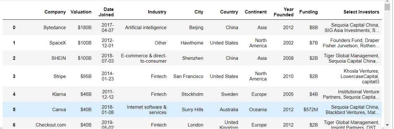
Examining the dataset

I used the df.info() function to check if the values are in a consistent format and can be appropriately used for analysis.

df.info()

The output of df.info() shows that the dataset contains 1074 entries with 10 columns. It appears that there are missing values in the 'Select Investors' and 'City' columns. Additionally, the data types for the 'Valuation', 'Date Joined', and 'Funding' columns are represented as objects instead of numerical values and standardized datetime format, which could potentially affect the accuracy of any calculations or analyses performed on these columns.

After inspecting the data types of each column in the data frame, I proceeded to apply the value_counts() method to each column to identify any potential data entry errors or formatting issues.

df['Valuation'].value_counts()

Upon inspecting the 'Valuation' column, I observed that the entries include a dollar sign $ and the letter B, indicating billions.

df['Industry'].value_counts()

From the Industry column, it can be observed that there are two categories for "Artificial Intelligence" with different capitalizations. This may lead to inconsistencies in the data and should be standardized to ensure accurate analysis.

df['Funding'].value_counts()

The 'Funding' column has entries with varying formats such as a dollar sign $, followed by a value and the letter B for billions, and M for millions. Additionally, there are some entries with the label Unknown which could potentially impact any analyses or calculations performed on this column.

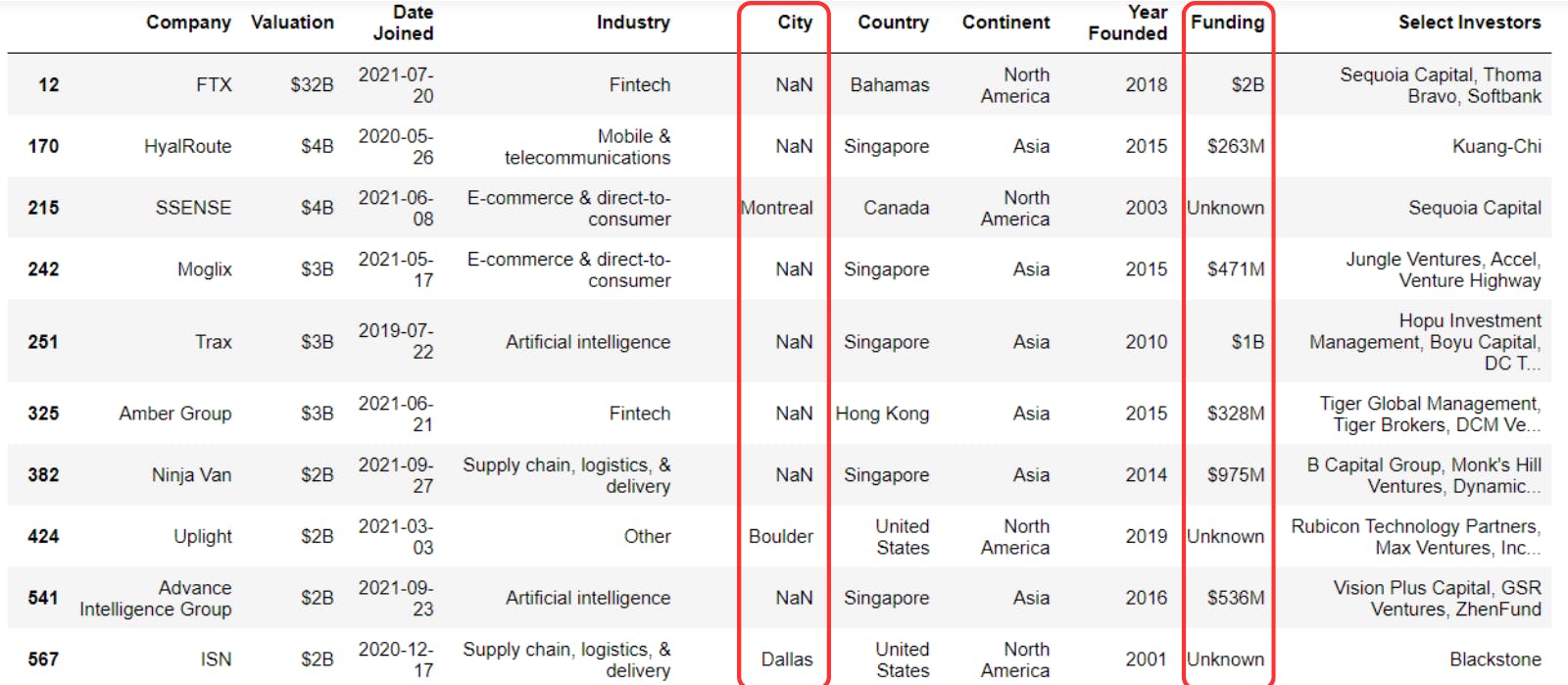
Identifying and handling missing values

During the initial exploration of the dataset, I identified two types of missing values: NaN values indicating the absence of data and entries labeled as Unknown indicating unidentified or unprovided values. Distinguishing between these two types was crucial since each required a different approach.

mask = df.isna() | (df == 'Unknown')
null_counts = mask.any(axis=1)
df[null_counts]

#  replace all 'Unknown' values in the 'Funding' column with NaN 
df['Funding'] = df['Funding'].replace('Unknown', np.nan)
# drop all rows containing NaN values in the 'Funding' column
df = df.dropna(subset=['Funding'])

# drop all rows in the DataFrame df that contain missing values NaN
df.dropna(inplace = True)

# reset the index 
df = df.reset_index(drop=True)

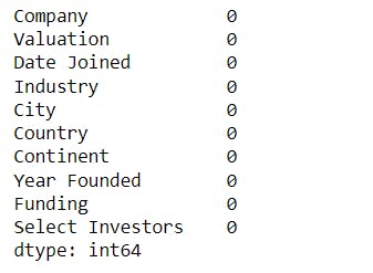
# Find missing values
df.isna().sum()

Correct data format

The next step in cleaning is checking and making sure that the data is in the correct format. In Pandas, we use.dtype() to check the data type, and .astype() to change the data type.

# Converting datatype of "Date Joined" to datetime datatype
df['Date Joined'] = df['Date Joined'].astype('datetime64')

To convert the data types of the remaining columns into the correct formats, it is necessary to first address the presence of characters such as $, B, and M in the 'Valuation' and 'Funding' columns. Neglecting this step will result in errors during the data type conversion process.

# Removing "$" and "B" from Valuation column
df.Valuation = df.Valuation.str.replace("$","", regex=False)
.str.replace("B",'0'*9, regex=False)

# Removing "$", "B", "M" and "Unknown" from Funding column
df.Funding = df.Funding.str.replace("$","", regex=False)
.str.replace("B",'0'*9, regex=False).str.replace("M",'0'*6, regex=False)

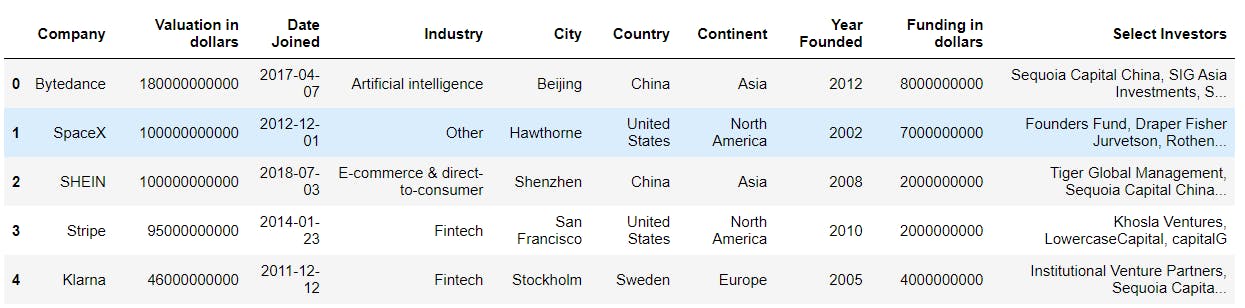
df.rename(columns = {'Funding': 'Funding in dollars', 'Valuation': 'Valuation in dollars'}, inplace= True)

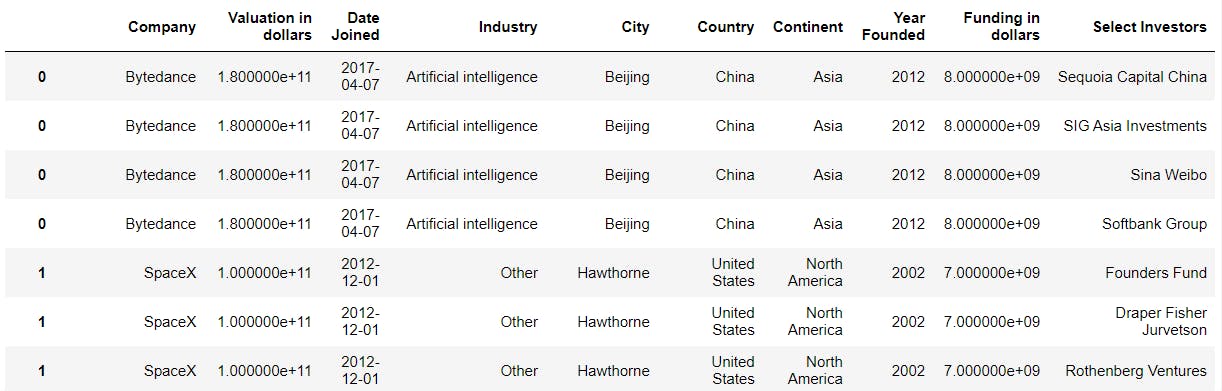
df.head(5)

# Converting Valuation and Funding columns to float type
df['Valuation in dollars'] = df['Valuation in dollars'].astype(float)
df['Funding in dollars'] = df['Funding in dollars'].astype(float)

Checking for duplicates

Checking for duplicates is an essential step in data analysis, if duplicates are not identified and removed, they can lead to overestimation or underestimation of certain values, resulting in inaccurate conclusions. Additionally, duplicate data can also cause issues with certain statistical analyses, such as correlation and regression, as they assume that each observation is independent. Therefore, it is crucial to check for duplicates and remove them to ensure the accuracy and reliability of the analysis results.

I began the process by initially applying the .duplicated() function to the entire DataFrame and then to each individual column.

duplicates = df.duplicated()
print("Number of duplicate rows:", duplicates.sum())

duplicates = df['Company'].duplicated()
print("Number of duplicate rows:", duplicates.sum())

df['Company'].value_counts().sort_index()

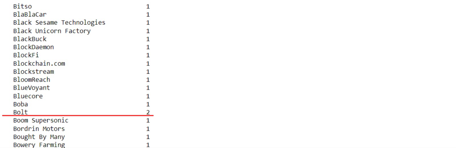
df[df["Company"] == "Bolt"]

I observed that there are duplicates of "Bolt" companies founded in different countries and belonging to different industries. To avoid confusion or errors in further analysis, I decided to differentiate the two companies by adding the country name in parentheses to their respective column names.

df.loc[40,"Company"] = 'Bolt (Estonia)'
df.loc[44,"Company"] = 'Bolt (United States)'

Also, to perform any analysis on the 'Select Investors' column, I needed to transform it first. It can be done by splitting the column into separate values wherever there is a comma followed by a space using the str.split(", ") method. Then, I used the explode() method to split the resulting list into multiple rows and duplicate the corresponding data in the other columns.

df["Select Investors"] = df["Select Investors"].str.split(", ")
df = df.explode("Select Investors")

# Group the data by Select Investors and count the number of unicorns each investor has funded
investor_counts = df.groupby('Select Investors')['Company'].count().sort_values(ascending=False)[:10]

# Create a vertical bar plot
plt.figure(figsize=(10,6))
sns.barplot(x=investor_counts.index, y=investor_counts.values, color='b')

# Add labels and title
plt.title('Top Investors by Number of Funded Unicorns')
plt.xlabel('Investor')
plt.ylabel('Number of Funded Unicorns')

# Rotate x-axis labels for readability
plt.xticks(rotation=90)

# Display the plot
plt.show()

To keep the reading simple and not exceed the scope of this post, I have left further analysis and visualization for another post, which will follow.

By applying these basic data wrangling techniques, we can obtain a cleaner dataset that is easier to work with and visualize. From here, we can dive deeper into the data to gain valuable insights and make data-driven decisions. Remember, data analysis is an iterative process, and the more we work with the data, the better our understanding becomes. I hope this post has provided some helpful tips and insights for your own data analysis projects.

Thank you for reading.